Category Archives: Wiki

What Is OpenFlow and How Does It Work?

OpenFlow is a communication protocol originally introduced by researchers at Stanford University in 2008. It allows the control plane to interact with the forwarding plane of a network device, such as a switch or router.

OpenFlow separates the forwarding plane from the control plane. This separation allows for more flexible and programmable network configurations, making it easier to manage and optimize network traffic. Think of it like a traffic cop directing cars at an intersection. OpenFlow is like the communication protocol that allows the traffic cop (control plane) to instruct the cars (forwarding plane) where to go based on dynamic conditions.

How Does OpenFlow Relate to SDN?

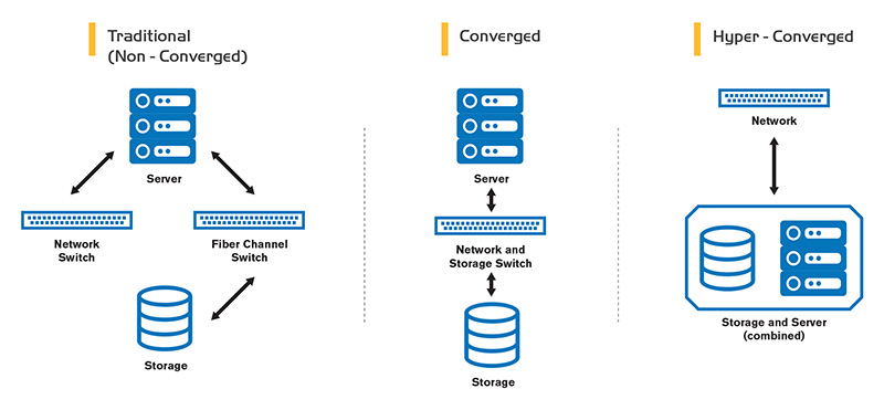
OpenFlow is often considered one of the key protocols within the broader SDN framework. Software-Defined Networking (SDN) is an architectural approach to networking that aims to make networks more flexible, programmable, and responsive to the dynamic needs of applications and services. In a traditional network, the control plane (deciding how data should be forwarded) and the data plane (actually forwarding the data) are tightly integrated into the network devices. SDN decouples these planes, and OpenFlow plays a crucial role in enabling this separation.

OpenFlow provides a standardized way for the SDN controller to communicate with the network devices. The controller uses OpenFlow to send instructions to the switches, specifying how they should forward or process packets. This separation allows for more dynamic and programmable network management, as administrators can control the network behavior centrally without having to configure each individual device.

” Also Check – What Is Software-Defined Networking (SDN)?

How Does OpenFlow Work?

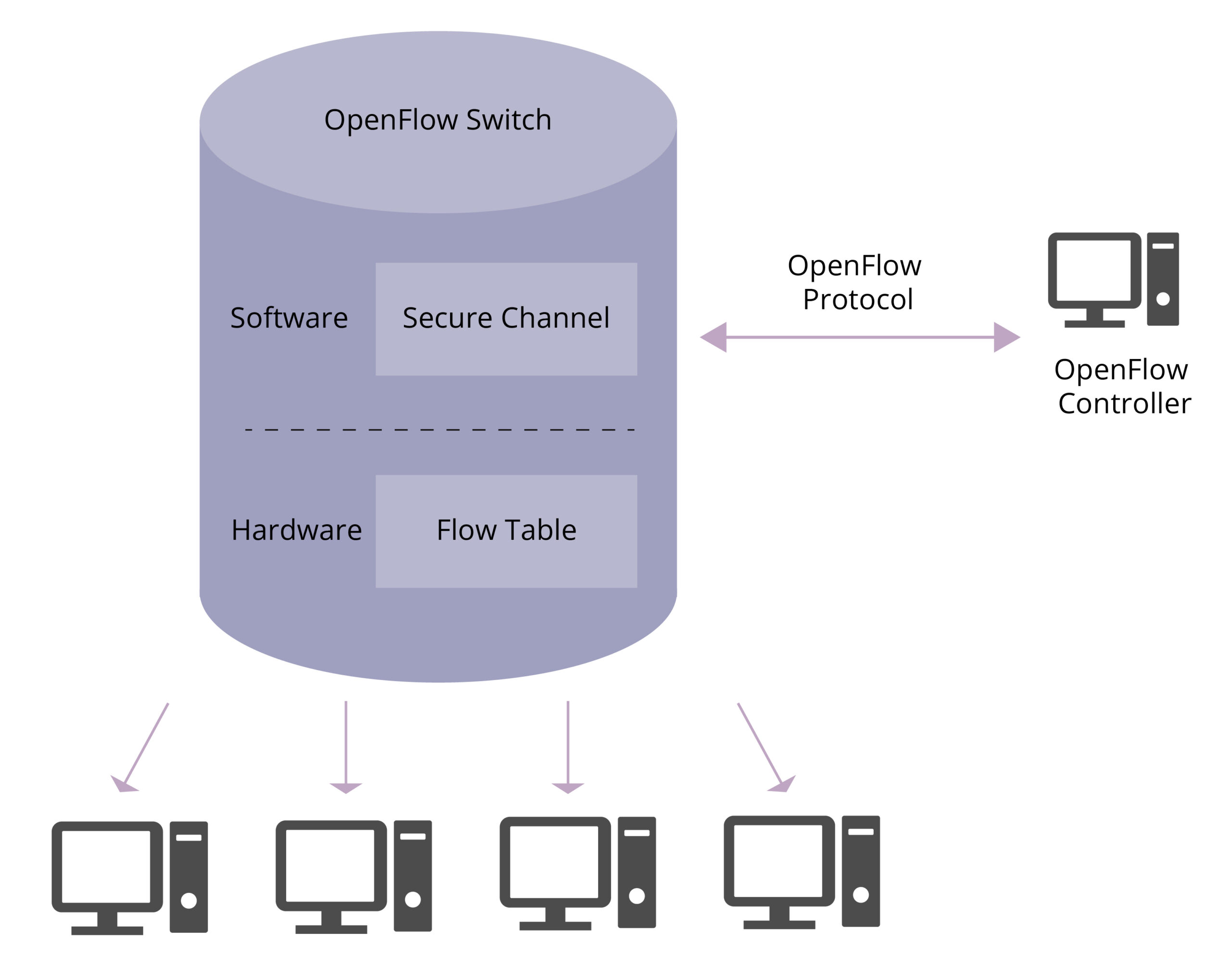
The OpenFlow architecture consists of controllers, network devices and secure channels. Here’s a simplified overview of how OpenFlow operates

Controller-Device Communication:

An SDN controller communicates with network devices (usually switches) using the OpenFlow protocol.
This communication is typically over a secure channel, often using the OpenFlow over TLS (Transport Layer Security) for added security.

Flow Table Entries:

An OpenFlow switch maintains a flow table that contains information about how to handle different types of network traffic. Each entry in the flow table is a combination of match fields and corresponding actions.

Packet Matching:

When a packet enters the OpenFlow switch, the switch examines the packet header and matches it against the entries in its flow table.
The match fields in a flow table entry specify the criteria for matching a packet (e.g., source and destination IP addresses, protocol type).

Flow Table Lookup:

The switch performs a lookup in its flow table to find the matching entry for the incoming packet.

Actions:

Once a match is found, the corresponding actions in the flow table entry are executed. Actions can include forwarding the packet to a specific port, modifying the packet header, or sending it to the controller for further processing.

Controller Decision:

If the packet doesn’t match any existing entry in the flow table (a “miss”), the switch can either drop the packet or send it to the controller for a decision.
The controller, based on its global view of the network and application requirements, can then decide how to handle the packet and send instructions back to the switch.

Dynamic Configuration:

Administrators can dynamically configure the flow table entries on OpenFlow switches through the SDN controller. This allows for on-the-fly adjustments to network behavior without manual reconfiguration of individual devices.

” Also Check – Open Flow Switch: What Is It and How Does It Work

What are the Application Scenarios of OpenFlow?

OpenFlow has found applications in various scenarios. Some common application scenarios include:

Data Center Networking

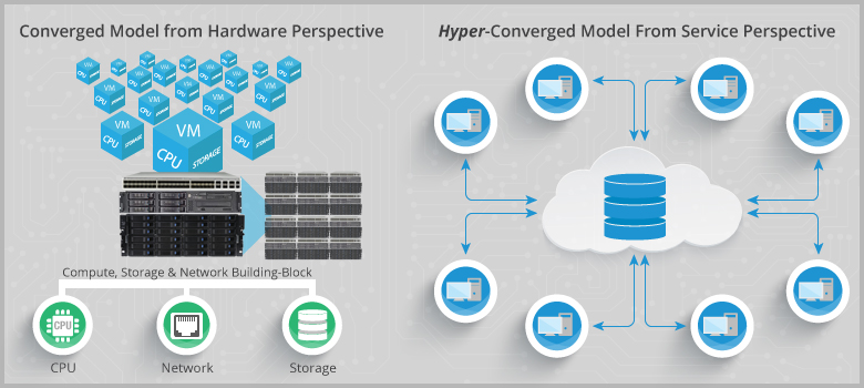
Cloud data centers often host multiple virtual networks, each with distinct requirements. OpenFlow supports network virtualization by allowing the creation and management of virtual networks on shared physical infrastructure. In addition, OpenFlow facilitates dynamic load balancing across network paths in data centers. The SDN controller, equipped with a holistic view of the network, can distribute traffic intelligently, preventing congestion on specific links and improving overall network efficiency.

Traffic Engineering

Traffic engineering involves designing networks to be resilient to failures and faults. OpenFlow allows for the dynamic rerouting of traffic in the event of link failures or congestion. The SDN controller can quickly adapt and redirect traffic along alternative paths, minimizing disruptions and ensuring continued service availability.

Networking Research Laboratory

OpenFlow provides a platform for simulating and emulating complex network scenarios. Researchers can recreate diverse network environments, including large-scale topologies and various traffic patterns, to study the behavior of their proposed solutions. Its programmable and centralized approach makes it an ideal platform for researchers to explore and test new protocols, algorithms, and network architectures.

In conclusion, OpenFlow has emerged as a linchpin in the world of networking, enabling the dynamic, programmable, and centralized control that is the hallmark of SDN. Its diverse applications make it a crucial technology for organizations seeking agile and responsive network solutions in the face of evolving demands. As the networking landscape continues to evolve, OpenFlow stands as a testament to the power of innovation in reshaping how we approach and manage our digital connections.

What’s the Current and Future Trend of 400G Ethernet?

According to the leading Cloud Service Providers (CSPs) and various networking forecast reports, 400G Ethernet will emerge as the leading technology since 2020. IDC (International Data Corporation) and Cignal Ai have also proved the similar situation. In short, 400G Ethernet will replace 100G and 200G deployments in a faster way than 100G did to the previous Ethernet.

Faster 400G Ethernet Trend Than Previous Ethernet.jpg

The Rise of 400G Ethernet

The factors affecting the development of 400G are mainly application-driven and technology-driven. The application drivers include 5G high-speed transmission, market requirements for data centers, cloud computing, and high-definition video transmission. Technology drivers include development of technologies in the market and product standardization.

Application-Driven Factors

5G Accelerates 400G Ethernet: An analysis from Cisco points out that 5G technology needs edge computing architecture, which brings cloud resources—compute, storage and networking—closer to applications, devices and users. While, the edge computing needs more bandwidth, support for more devices on the network, and greater security to protect and manage the data. For example, a 4G radio system can support up to only 2,000 active devices in a square kilometer, while 5G could support up to 100,000 active devices in the same range. With 400G technology offering more bandwidth, more devices and applications could be supported in 5G.

ITEMS	4G LTE	5G
Average Data Rate	25 Mb/s	100 Mb/s
Peak Data Rate	150 Mb/s	10,000 Mb/s
Latency	50 ms	1 ms
Connection Density	2,000 Per Square Kilometer	100,000 Per Square Kilometer

Data Center & Cloud Computing Requirements: A research from Cisco indicates that cloud-based data centers will take over 92% of the next-generation data center workload while the traditional data centers will take over less than 8% after 2021. These objective requirements for higher data rates drive 400G development greatly. It is estimated that 400G will be the prevailing speed in switch chips and network platforms in the coming years.
High-Definition Video Transmission Needs: Basically all forms of Internet applications are moving towards video. It is estimated that more than 80% of the traffic is video. Video is a very important platform for everyone to interact in the future, especially real-time video streaming, such as multi-party video conferences. High-definition videos (such as 4K videos) need more bandwidth and less latency compared with the previous normal ones featuring lower definition.

Technology-Driven Factors

400G technology was originally known as IEEE 802.3bs and was officially approved in December, 2017. It regulates new standards including Forward Error Correction (FEC) to improve error performance. Abide by these standards, early 400G network elements have successfully completed trials and initial deployment. At present, some brand 400G switches have been put into use such as Cisco 400G Nexus, Arista 400G 7060X4 Series, Mellanox Spectrum-2, FS 400G switch, etc. 400G connection scheme is also blooming such as 400G DAC and 400G transceivers (400G QSFP-DD transceiver, 400G OSFP transceiver, 400G CFP8 transceiver, etc.), of which 400G QSFP-DD is becoming the leading form factor for its high density and low power consumption. As 400G Ethernet grows faster to standardization, commercialization and scale, soon 400G product system will be gradually perfect and more 400G products will appear in return.

Influences of 400G Ethernet

400G Optics Promotes 25G and 100G Markets While Reduces 200G Market Share

Compared to the 10G Ethernet, 25G Ethernet gains more popularity in the whole optical transmission industry because 25Gbps and 50Gbps per channel technology provide the basic standards for existing 100G (4x 25Gbps), the coming 400G (8x 50Gbps) and the future 800G network. Therefore, the rapid development of 400G Ethernet will promote the 25G and 100G markets to a certain extent in turn. Similarly, the quick appearance of 400G applications implicates that 200G is a flash in the pan.

400G Technology Is Expected to Reduce Overall Network Operation and Maintenance Costs

For access, metro, and data center interconnection scenarios, where short transmission distance and higher bandwidth are required, fiber resources are relatively scarce. The single-carrier 400G technology can provide the largest transmission bandwidth and the highest spectral efficiency with the simplest configuration, which effectively reduces transmission costs.
In the backbone and some more complex metropolitan area networks, where the transmission distance is longer with more network nodes, the requirements for transmission performance are more stringent. Under such circumstances, dual-carrier technology (2x 200G) and an optimized algorithm could work together to compress the channel spacing. This can not only improve the spectral efficiency by 30% (close to the level of a single-carrier 400G technology), but also extend the transmission distance of 400G Ethernet to several thousand kilometers, helping operators quickly deploy 400G backbone networks with minimum bandwidth resources.
400G solution can also increase the single fiber capacity by 40% and reduce power consumption by 40%, thereby greatly improving network performance and reducing network operation and maintenance costs.

Opportunities for 400G Ethernet Vendors and Users

Many suppliers hype their 400G products to get ahead of the curve. Actually, few vendors have the real supply capacity and the quality of most 400G products supplied can’t be assured. To win from the fierce market competition, vendors should pay more attention to improving product quality and strong supply capability. And this is indubitably beneficial to users, who can get better products and services with relatively lower prices.

Impact of 400G Optics on Cabling and Connectivity

In the multimode installed base, the biggest difference between 100G and 400G modules is the increase in total number of fibers. For single mode transmission system, most of the duplex LC and MPO-based architecture that is deployed at 100G should serve for 400G. For parallel or multi-fiber transmission, transceivers like 400GBASE-SR4.2 operating with short wavelength division multiplexing (SWDM) at four wavelengths provide longer distances over OM5 fiber than OM4 or OM3. And OM5 wideband multimode fiber (WBMMF) will allow use of SWDM technology to transmit multiple signals (wavelengths) on one fiber. This indicates that OM5 fiber and SWDM technologies will continue to offer improved support on 400G Ethernet.

Are You Ready for 400G Ethernet?

400G Ethernet is an inevitable trend in current networking market. Driven by various market demands and technologies, it has come more rapidly than any previous technology. And it also has many significant effects, such as reducing the market share of 200G and saving transmission costs to a certain extent. There are already some mature 400G optics products in the market, such as 400G QSFP-DD transceivers, 400G DACs, as well as 400G DAC breakout cables. And 400G technology is no doubt going to be more and more advanced to promote the developments of 400G Ethernet and 400G applications.

Original Source: What’s the Current and Future Trend of 400G Ethernet?

NRZ vs. PAM4 Modulation Techniques

The leading trends such as cloud computing and big data drive the exponential traffic growth and the rise of 400G Ethernet. Data center networks are facing a larger bandwidth demand, and innovative technologies are required for infrastructure to meet shifting demands. Currently, there are two different signal modulation techniques examined for next-generation Ethernet: non-return to zero (NRZ), and pulse-amplitude modulation 4-level (PAM4). This article will take you through these two modulation techniques and compare them to find the optimal choice for 400G Ethernet.

NRZ and PAM4 Basics

NRZ is a modulation technique using two signal levels to represent the 1/0 information of a digital logic signal. Logic 0 is a negative voltage, and Logic 1 is a positive voltage. One bit of logic information can be transmitted or received within each clock period. The baud rate, or the speed at which a symbol can change, equals the bit rate for NRZ signals.

PAM4 is a technology that uses four different signal levels for signal transmission and each symbol period represents 2 bits of logic information (0, 1, 2, 3). To achieve that, the waveform has 4 different levels, carrying 2 bits: 00, 01, 10 or 11, as shown below. With two bits per symbol, the baud rate is half the bit rate.

Comparison of NRZ vs. PAM4

Bit Rate

A transmission with NRZ mechanism will have the same baud rate and bitrate because one symbol can carry one bit. 28Gbps (gigabit per second) bitrate is equivalent to 28GBdps (gigabaud per second) baud rate. While, because PAM4 carries 2 bits per symbol, 56Gbps PAM4 will have a line transmission at 28GBdps. Therefore, PAM4 doubles the bit rate for a given baud rate over NRZ, bringing higher efficiency for high-speed optical transmission such as 400G. To be more specific, a 400 Gbps Ethernet interface can be realized with eight lanes at 50Gbps or four lanes at 100Gbps using PAM4 modulation.

Signal Loss

PAM4 allows twice as much information to be transmitted per symbol cycle as NRZ. Therefore, at the same bitrate, PAM4 only has half the baud rate, also called symbol rate, of the NRZ signal, so the signal loss caused by the transmission channel in PAM4 signaling is greatly reduced. This key advantage of PAM4 allows the use of existing channels and interconnects at higher bit rates without doubling the baud rate and increasing the channel loss.

Signal-to-noise Ratio (SNR) and Bit Error Rate (BER)

According to the following figure, the eye height for PAM4 is 1/3 of that for NRZ, causing the PAM4 to increase SNR (Signal-Noise Ratio) by -9.54 dB (Link Budget Penalty), which impacts the signal quality and introduces additional constraints in high-speed signaling. The 33% smaller vertical eye opening makes PAM4 signaling more sensitive to noise, resulting in a higher bit error rate. However, PAM4 was made possible because of forward-error correction (FEC) that can help link system to achieve the desired BER.

Power Consumption

Reducing BER in a PAM4 channel requires equalization at the Rx end and pre-compensation at the Tx end, which both consume extra power than the NRZ link for a given clock rate. This means PAM4 transceivers generate more heat at each end of the link. However, the new state-of-the-art silicon photonics (SiPh) platform can effectively reduce energy consumption and can be used in 400G transceivers. For example, FS silicon photonics 400G transceiver combines SiPh chips and PAM4 signaling, making it a cost-effective and lower power consumption solution for 400G data center.

Shift from NRZ to PAM4 for 400G Ethernet

With massive data transmitted across the globe, many organizations pose their quest for migration towards 400G. Initially, 16× 25G baud rate NRZ is used for 400G Ethernet, such as 400G-SR16, but the link loss and size of the scheme can not meet the demands of 400G Ethernet. Whereas PAM4 enables higher bit rates at half the baud rate, designers can continue to use existing channels at potential 400G Ethernet data rates. As a result, PAM4 has overtaken NRZ as the preferred modulation method for electrical or optical signal transmission in 400G optical modules.

Article Source: NRZ vs. PAM4 Modulation Techniques

An Overview on EVPN and LNV

Bombarded with assorted network applications and protocols, the technologies and solutions for network virtualization delivery have been enriched greatly over past years. Among those technologies, VXLAN, also called virtual extensible local area network, is the key network virtualization. It enables layer 2 segments to be extended over an IP core (the underlay). The initial definition of VXLAN (RFC 7348) only relied on a flood-and-learn approach for MAC address learning. Now, a controller or a technology such as EVPN and LNV in Cumulus Linux can be realized. In this post, we are going to make an exploration on those two techniques: LNV and EVPN.

Figure 1: VXLAN

What Is EVPN

EVPN is also named as Ethernet VPN. It is largely considered as a unified control plane solution for the controller-less VXLAN, allowing for building and deploying VXLANs at scale. The EVPN relies on multi-protocol BGP (MP-BGP) to transport both layer 2 MAC and layer 3 IP information at the same time. It enables a separation between the data layer and control plane layer. By having the combined set of MAC and IP information available for forwarding decisions, optimized routing and switching within a network becomes feasible and the need for flooding to do learning gets minimized or even eliminated.

What Is LNV

LNV is the short of lightweight network virtualization. It is a technique for deploying VXLANs without a central controller on bare metal switches. Typically, it’s able to run the VXLAN service and registration daemons on Cumulus Linux itself. The data path between bridge entities is established on the top of a layer 3 fabric by means of a simple service node coupled with traditional MAC address learning.

The Relationship Between EVPN and LNV

From the above wiki of the EVPN and LNV, it’s easy for us to notice these two technologies are both the applications of VXLAN. For LNV, it can be used to deploy VXLAN without an external controller or software suite on the bare-metal layer 2/3 switches running Cumulus Linux network operating system (NOS). As for EVPN, it is a standards-based control plane for VXLAN, which can be used in any usual bare-metal devices, such as network switch and router. Typically, you cannot apply LNV and EVPN at the same time.

Apart from that, the deployments for EVPN and LNV are also different. Here, we make a configuring model for each of them for your better visualization.

EVPN Configuration Case

Figure 2: EVPN

In the EVPN-VXLAN network segments shown in Figure 2 (Before), hosts A and B need to exchange traffic. When host A sends a packet to host B or vice versa, the packet must traverse the switch A, a VXLAN tunnel, and the switch B. By default, routing traffic between a VXLAN and a Layer 3 logical interface is disabled. If the functionality is disabled, the pure Layer 3 logical interface on the switch A drops Layer 3 traffic from host A and VXLAN-encapsulated traffic from the switch B. To prevent the pure Layer 3 logical interface on the switch A from dropping this traffic, you can reconfigure the pure Layer 3 logical interface as a Layer 2 logical interface, like Figure 2 (After). After that, you need to associate this interface with a dummy VLAN and a dummy VXLAN network identifier (VNI). Then, an Integrated routing and bridging (IRB) interface need to be created, which provides Layer 3 functionality within the dummy VLAN.

LNV Configuration Case

Figure 3: LNV

The two layer 3 switches are regarded as leaf 1 and leaf 2 in the above figure. They are running with Cumulus Linux and have been configured as bridges. Containing physical switch port interfaces, the two bridges connect to the servers as well as the logical VXLAN interface associated with the bridge. After creating a logical VXLAN interface on both leaf switches, the switches become VTEPs (virtual tunnel end points). The IP address associated with this VTEP is most commonly configured as its loopback address. In the image above, the loopback address is 10.2.1.1 for leaf 1 and 10.2.1.2 for leaf 2.

Summary

In this post, we have introduced the two techniques of network virtualization: EVPN and LNV. These two applications of network virtualization delivery share some similarities, but also quite a lot of differences. Being satisfied with the simplicity, agility, and scalability over the network, the EVPN has been a popular choice in the market.

Hyper Converged Infrastructure vs Converged Infrastructure

Hyper converged infrastructure has been talked a lot in recent years and its adoption is skyrocketing in data centers. However, many people are still confused by this term. Converged Infrastructure vs hyper converged infrastructure, what’s the difference between them? This post will introduce it in details.

What’s Hyper Converged Infrastructure

Hyper converged infrastructure is often named HCI. It is introduced in 2012 to describe a fully software-defined IT infrastructure that virtualizes all the elements of conventional hardware-defined systems. In other words, the networking and storage tasks in the hyper converged infrastructure are implemented virtually through software rather than physically in hardware. Generally, hyper converged infrastructure is at least composed of virtualized computing (a Hypervisor), a virtualized SAN (software-defined storage) and virtualized networking (Software-defined networking). It can be utilized as a way to pool together resources so as to maximize the interoperability of on-premises infrastructure.

Hyperconverged Infrastructure

Hyper Converged Infrastructure vs Converged Infrastructure

Hyper converged infrastructure and converged infrastructure are two alternative solutions to replace the traditional IT infrastructure. This part will tell the differences between them to help you choose one over another for your network deployment.

converged infrastructure vs hyper converged infrastructure

Hyper Converged vs Converged Infrastructure Components

Converged infrastructure defines compute, storage, networking and server virtualization—which are the four core components in a data center—as one dense building block. Hyperconverged infrastructure is born from converged infrastructure and the idea of the software-defined data center (SDDC). Besides the data center’s four core components, hyperconverged infrastructure integrates more components such as backup software, snapshot capabilities, data deduplication, inline compression, WAN optimization and so on.

Hyper Converged vs Converged Infrastructure Principle

Hyper converged infrastructure is a software defined approach. It means the infrastructure operations are logically separated from the physical hardware, and all components in a hyper converged infrastructure have to stay together to function correctly. While converged infrastructure is a hardware-focused, building-block approach. Each component in a converged infrastructure is discrete and can be used for its intended purpose. For example, the server can be separated and used as a server, just as the storage can be separated and used as functional storage.

Hyperconverged VS Converged Infrastructure Principle

Hyper Converged vs Converged Infrastructure Cost

Converged infrastructure allows IT to use a single vendor for end-to-end support for all core components instead of the traditional approach where IT might buy storage from one vendor, network from another and compute from another. It also offers a smaller footprint and less cabling, which can reduce the cost of installation and maintenance.

Hyper converged infrastructure allows IT to build, scale and protect your IT infrastructure more affordably and effectively. For example, a 10GbE Access Layer Switch (8*10/100/1000Base-T+8*1GE SFP Combo+12*10GE SFP+) specially for hyper converged infrastructure only costs US$ 1,699. And the software-defined intelligence reduces operational management, providing automated provisioning of compute and storage capacity for dynamic workloads.

Conclusion

It is reported that hyper converged infrastructure will represent over 35 percent of total integrated system market revenue by 2019. This makes it one of the fastest-growing and most valuable technology segments in the industry today. The upfront costs of hyper converged infrastructure may be a little high now, but in the long term it can pay off.

Tutorials Of Fiber Optic Products

Here You Can Find The Best Fiber Optic Tutorials!